TSNE降维可视化
工作中遇到了高维度数据可视化的需求,之前没有做类似的任务,记录一下学习的过程。
几个问题
问题一:为什么需要做高维度数据可视化?
想通过产生的图,去观察或者说去猜测一些数据是否有联系,能不能找出一些规律,去做一个假设。问题二:选用什么方法去做可视化?
在Google中搜索高维度数据可视化,搜索到的结果有ISOMAP(等度量映射)、PCA(主成分分析)、T-SNE等,其中很多都提到了T-SNE效果好,并给出了Digits数据集的例子。通过测试Digits数据集得到的效果,决定选用T-SNE去实现。问题三:怎么实现?
在scikit-learn中已经实现了T-SNE的算法,并给出了官方代码示例,直接使用即可。
简述T-SNE
T-SNE(T-Distribution Stochastic Neighbour Embedding, T分布随机近邻嵌入),一种用于降维的机器学习算法,另外,它是一种非线性降维算法,非常适用于将高维数据降维到2维或者3维进行可视化。
我不是算法工程师,也不是机器学习工程师,具体的算法实现是真的看不懂,就只把论文和部分资料链接放在这里好了:
T-SNE论文: http://www.jmlr.org/papers/v9/vandermaaten08a.html
部分中文文章对T-SNE的介绍:
详解可视化利器 t-SNE 算法:数无形时少直觉
https://www.zhihu.com/question/52022955/answer/387753267
scikit-learn文档中TSNE的各参数含义:
https://scikit-learn.org/stable/modules/generated/sklearn.manifold.TSNE.html
这里也提到了T-SNE的优缺点:
https://scikit-learn.org/stable/modules/manifold.html#t-sne
在我实际使用中,的确感受到了计算成本很高这一点,是真的慢…
简述Digits
scikit-learn中自带的Digits数据集由1797个图像数据矩阵组成,每个数据点都是0到9之间手写数字的一张8×8灰度图像。
那么引入代码看一下:
1 | from sklearn.datasets import load_digits |
其中:
digits.data:手写数字的特征向量
digits.target:特征向量对应的标记,每一个元素都是0-9的数字
digits.images:提供了images表示,与data中数据一致,只是转变为8*8的数组表示
1 | # 查看数据集的形状 |
使用T-SNE
官方使用Digits数据集和各算法进行计算的代码示例:
https://scikit-learn.org/stable/auto_examples/manifold/plot_lle_digits.html#sphx-glr-auto-examples-manifold-plot-lle-digits-py
我把代码稍微修改了一下,比较简单,使用matplotlib来生成二维和三维图片
1 | import numpy as np |
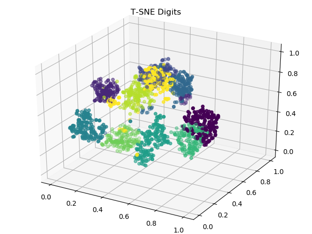
实现效果
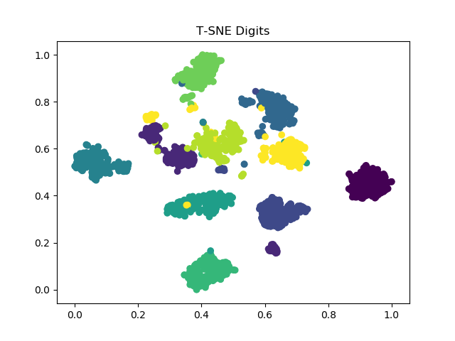
三维图片的保存还没学会,先这么凑合着看(逃
另外,关于相关参数对结果的影响,可以查看:
https://scikit-learn.org/stable/auto_examples/manifold/plot_t_sne_perplexity.html#sphx-glr-auto-examples-manifold-plot-t-sne-perplexity-py
https://distill.pub/2016/misread-tsne/
学习的过程大致就是这样啦,只不过实际工作中使用的数据不一样,思路上是一样的。